Virtual machine deployment and scaling workflows

• How the persistent storage VMs function under different workflows

• Configured network and tuned profiles
• Red Hat Ceph Storage deployed
• Red Hat OpenShift deployed
• Virtual machines configured and cloned

Effective VM deployment forms the foundation of any virtual environment, especially when operating at a high scale. The expeditious deployment of a substantial number of VMs directly impacts the efficiency of our production processes.

Within this section, we will elucidate the performance benchmarks attainable through the cloning of multiple VM images from a golden image source, employing the snapshot cloning method. This analysis aims to shed light on the deployment efficiency and potential outcomes for our virtual infrastructure.

End-to-End Deployment

The provided chart showcases the duration of VM deployment, which is the VM object and PVC creation. The tests gradually increased the number of RHEL VMs deployed, starting with 100 and doubling in size every test, ultimately reaching 6000 VMs. The deployment is done in parallel for every bulk.

Following each deployment, all VMs were deleted to ensure a clean setup for subsequent tests.

The chart's findings demonstrate a notable trend, revealing near-linear deployment behavior. Each test's duration is approximately twice that of its predecessor, highlighting a consistent pattern of scalability as the number of VMs increases. This observation underscores the system's efficiency in handling larger VM quantities, showcasing promising and predictable deployment performance.

Per VM Deployment

In this scenario, the emphasis was shifted from large bulk VM deployments to a detailed examination of individual VM deployment times. The primary objective was to verify the absence of any underlying issues during the deployment process.

The provided charts display the individual percentile metrics for VMs, offering a comprehensive view of the deployment durations for each VM. By assessing these individual metrics, we gain valuable insights into the variability and distribution of VM deployment times. This analysis enables us to identify potential outliers and ensure that the deployment process is stable and efficient for all individual VMs.

VMs Boot Storm

In this section, we conducted a comprehensive test to assess the boot times of a substantial number of virtual machines (VMs), a scenario often encountered in disaster recovery situations such as power outages or planned hardware maintenance. Additionally, a key objective was to evaluate whether the VMs were evenly distributed across the cluster during the booting process.

End-to-End Boot Time

In this test, we conducted a series of experiments involving the simultaneous booting of varying numbers of VMs, starting with 100 VMs and doubling the quantity with each subsequent test, eventually reaching 6000 VMs. The metric we used for evaluation was the time it took from initiating the boot request for each VM until it became accessible via SSH.

It's important to note that all the VM boot requests were launched in parallel, intentionally stressing all components of the cluster simultaneously. Following the measurement of each bulk of VMs, we systematically shut down all VMs before initiating the next batch.

The resulting chart reveals a remarkable display of near-linear parallelism, particularly evident up to the point of booting 1,600 VMs in parallel. This achievement showcases the cluster's impressive capability to efficiently handle increasing workloads without significant bottlenecks.

However, a notable turning point occurs at 3200 VMs, as observed in the chart, where we begin to notice a deviation from linear parallelism. This deviation is attributed to the buildup of queues, leading to a gradual increase in boot times. This finding underscores the importance of monitoring and optimizing the system's performance as it scales to such high levels, highlighting the complexity and challenges associated with managing large-scale parallel operations.

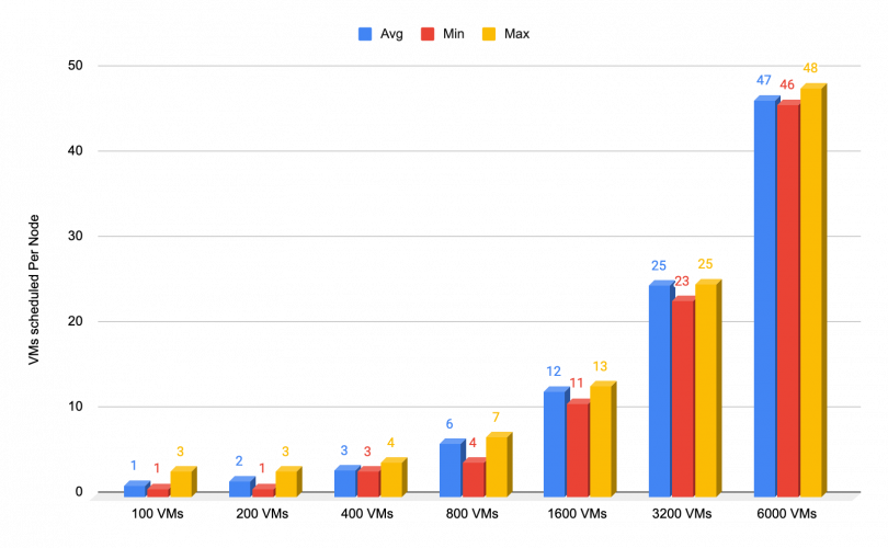
Scheduler

The following chart depicts the distribution of scheduled VMs across worker nodes within the cluster during the booting process of a large number of VMs. Ideally, we aim for an even distribution of VMs across all worker nodes. However, given the coexistence of other microservices within the cluster alongside VMs, the scheduling can be influenced.

The chart presents the average, minimum, and maximum number of VMs scheduled per node for each bulk test conducted.

Notably, the results indicate an exceptional outcome, signifying successful and balanced VM scheduling across the cluster. This achievement is particularly noteworthy considering the potential impact of concurrent microservices on the scheduling process.

VMs IO scaling

Introduction

In this scenario, we stress both the VMs and the network. To ensure the reliability of the test results, we imposed a total throughput constraint of 10 GiBs. This limitation was chosen to emulate a mid-high range throughput, while still allowing a high burst of small blocks, allowing us to assess if and to what extent the VM scaling impacts the performance. We used the 4KiB (CPU Intensive) and the 64KiB block size (Network Intensive) in order to achieve the above. We are using a 100% random pattern in order to prevent any caching from occurring.

Before running any test, we first created a baseline for comparison. The baseline measures the roundtrip latency for every VM by running a single IO of the same size against the VM disk giving us our baseline for the comparison.

All tests start with a single VM per worker node - meaning the first test will always start with 129 VMs since we have 129 worker nodes, and then progressively double the number of VMs per node, meaning 2 VMs per node or 258 VMs, and then 4 VMs per node and so on. This distributes the workload evenly across the cluster, which makes the results on this large scale repetitive and viable.

When it comes to read performance, a higher IOPS/throughput rate will yield lower latency in comparison to idle latency to some extent. This happens due to the resource allocation that occurs during high bursts when compared to idle/low IOPS workload on the VM. n this setup, the VMs are configured for the most common scenario in which the VMs are requesting resources (CPU/RAM) but do not hold on to them when Idle. They release those resources so that they are available to other VMs/components on the node. This role also applies to the Red Hat Ceph Storage pods that are running on the Red Hat Ceph Storage cluster, so when running a low demanding workload such as our baseline we do not trigger that resource allocation which results in higher latency than during burst testing.

Since the throughput limit has been set to a maximum of 10GiB’s that also limits the maximum IOPS to 2.6M when using the 4KiB block size, which gives us the bandwidth to stress both the CPU and network.

Each VM's filesystem dataset comprises 140 directories, each housing 15 files, with individual file sizes of 5MiB. To provide perspective, each VM held a 10.5 GiB dataset, culminating in a collective dataset size of 21.1 TiB for all 2064 VMs during the final test.

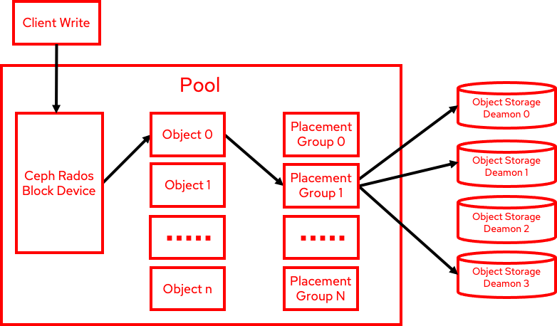
It's crucial to highlight that write operations follow a distinct data flow, which is essential for maintaining robust availability. With each write action, Red Hat Ceph Storage generates three data copies, transmitted through the network to their respective object storage daemons (OSDs). Consequently, write throughput consistently yields lower outcomes, while write latency invariably registers higher results compared to read operations, as illustrated in the accompanying diagram:

CPU intensive reads

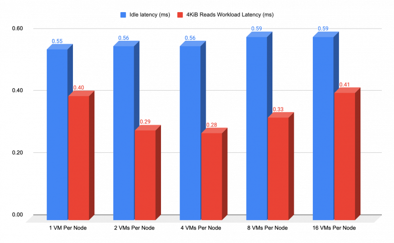
The chart below showcases the read IOPS results, where we used a block size of 4 KiB to exert maximum CPU stress on the VMs and ascertain that none of them or any other moving parts of the cluster encountered any interruptions while scaling up the number of VMs that are generating the workload.

As we mentioned earlier, in terms of read performance, there is a noticeable decrease in latency compared to the idle latency, albeit to a certain extent. This reduction is attributed to the resource allocation that takes place during the burst. The chart's results effectively illustrate this behavior starting at 129 VMs or 1 VM per node, up to 2064 VMs.

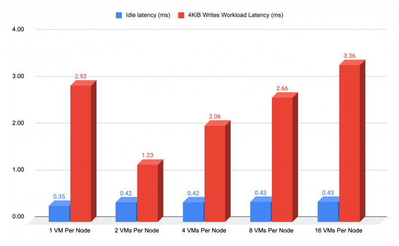
CPU intensive Writes

The chart below showcases the write IOPS results, whereby a block size of 4 KiB was employed to exert maximum CPU stress on the VMs. However, as previously mentioned, writes are less efficient due to the Red Hat Ceph Storage architecture, resulting in steadily increasing latency costs as we increase the number of clients (VMs) that are generating IO. That being said, these tests are only meant to uncover any issues that might occur under those conditions, but the probability of having 2064 VMs that suddenly erupt with that kind of IO burst is unlikely to happen on a real production.

VM disks are distributed across the Object Storage Devices (OSDs) within the Red Hat Ceph Storage cluster to ensure high availability (HA). In specific situations, such as the initial test shown on the chart, when the workload is executed with fewer VMs, we may observe occasional spikes in latency. This phenomenon occurs due to data distribution across a limited number of OSDs, thereby creating a bottleneck within those OSDs.

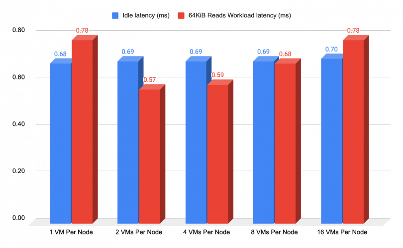
Network intensive reads

The chart below showcases the read throughput results, where we used a  block size of 64 KiB to exert network stress on the Network. As previously mentioned, when it comes to reads performance, a higher IOPS rate will yield lower latency to some extent due to the resource allocation that occurs during high bursts, as illustrated on the following chart:

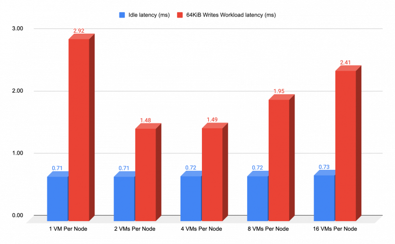
Network intensive writes

The same basic concepts for throughput results was applied in testing the latency of each VM under writing workload stress. The chart below showcases the results, where we used a  block size of 64 KiB to exert network stress on the Network. As we previously mentioned, when it comes to writes performance, a higher IOPS rate will yield lower latency to some extent.

• Troubleshoot with Red Hat support