
Red Hat blog
The new Multi-Instance GPU (MIG) feature lets GPUs based on the NVIDIA Ampere architecture run multiple GPU-accelerated CUDA applications in parallel in a fully isolated way. The compute units of the GPU, as well as its memory, can be partitioned into multiple MIG instances. Each of these instances presents as a stand-alone GPU device from the system perspective and can be bound to any application, container, or virtual machine running on the node. At the hardware-level, the MIG instance has its own dedicated resources (compute, cache, memory), so the workload running in one instance does not affect what is running on the other ones.
In collaboration with NVIDIA, we extended the GPU Operator to give OpenShift users the ability to dynamically reconfigure the geometry of the MIG partitioning (see Multi-Instance GPU Support with the GPU Operator v1.7.0 blog post). The geometry of the MIG partitioning is the way hardware resources are bound to MIG instances, so it directly influences their performance and the number of instances that can be allocated. The A100-40GB, which we used for this benchmark, has eight compute units and 40 GB of RAM. When the MIG mode is enabled, the eighth instance is reserved for resource management.
Here is a summary of the MIG instance properties of the NVIDIA A100-40GB product:
|
MIG Name |
MIG Instance Memory |
MIG Instance Compute Units |
Maximum number of homogeneous instances |
|
1g.5gb |
5 GB |
1 |
7 |
|
2g.10gb |
10 GB |
2 |
3 |
|
3g.20gb |
20 GB |
3 |
2 |
|
4g.20gb |
20 GB |
4 |
1 |
|
7g.40gb |
40 GB |
7 |
1 |
In addition to homogeneous instances, some heterogeneous combinations can be chosen. See NVIDIA documentation for the exhaustive listing, or refer to our previous blog post for OpenShift configuration.
Here is an example, again for the A100-40GB, with heterogeneous (or “mixed”) geometries:
- 2x 1g.5gb
- 1x 2g.10gb
- 1x 3g.10gb
Our work in the GPU Operator consisted of enabling OpenShift cluster administrator to decide the geometry to apply to the MIG-capable GPUs of a node, apply a specific label to this node, and wait for the GPU Operator to reconfigure the GPUs and advertise the new MIG devices as resources to Kubernetes.
In the remainder of this post, we go through the performance benchmarking we performed in parallel with this work to better understand the performance of each MIG instance size, and to validate the isolation of workloads running on different MIG instances of the same GPU in an OpenShift worker node.
Performance Benchmarking With MLPerf SSD
MLPerf is a consortium of key contributors from the AI/ML (Artificial Intelligence and Machine Learning) community that provides unbiased AI/ML performance evaluations of hardware, software, and services. In this work, we used NVIDIA PyTorch implementation of the Single Shot MultiBox Detector (SSD) training benchmark, from the MLPerf 0.7 repository. What follows is a study of the performance achieved by each MIG instance type. Then we look at the efficiency when multiple training workloads are running in parallel in different MIG instances (of the same sizes).
All the results presented in this post were executed on a Dell PowerEdge R7425 AMD Naples server (2x AMD EPYC 7601 32-Core processors, 512GB of RAM, 1.6TB SSD PCIe PM1725a Samsung disk) running with RHCOS 47.83 / Linux 4.18.0-240.10.1.el8_3 (OpenShift 4.7), with a A100-40GB PCIe GPU. The SSD benchmark ran against the full COCO dataset, with the default parameters from MLCommons repository. The only modification was that we requested more evaluation points (--evaluation 5 10 15 20 25 30 35 40 50 55 60 65 70 75 80 85), so that we could record the progress of the training over the time. The benchmark used the default quality target threshold: 0.23.
Each of the benchmarks were executed three times.
Performance of the Different MIG Instance Sizes
In the first part of this benchmarking study, we wanted to better understand the performance of each type of MIG instance. To measure this performance indicator, we ran an identical workload on each of the possible instance size of the A100-40GB GPU (including the full GPU, for reference):
- 1g.5gb (smallest)
- 2g.10gb
- 3g.20gb
- 4g,20gb
- 7g.40gb (biggest MIG instance)
- 8g.40gb (full GPU, MIG disabled)

Evolution of the Classification Threshold over the time, for the different MIG instances.
This plot shows the time the benchmark took (Y axis, in hours, lower is better) to reach a given image classification threshold, with the final target being 0.23. The main line shows the median value of the three executions, and the colored surface shows the standard deviation.

Time to reach the target threshold (0.23), for the different MIG instances.
This plot shows the time the benchmark took to reach the target classification threshold (red points, lower is better). The blue points show the perfect scaling times (that is, double the number of compute units, halve the execution time). The text labels indicate how much faster the actual benchmark was (higher is better).

Processing speed of the different MIG instances.
The red dots of this plot show the average number of image samples processed every second (as reported by the benchmark). Higher is better. The blue dots show the perfect scaling speeds (that is, double the number of compute units, double the processing speed). The text labels indicate the percentage of the perfect scaling speed was obtained during the benchmark execution (higher is better).
In these performance plots, we see that the MIG instance types directly influence the performance of the benchmark. This correlation between the number of GPU engines and the processing speed shows that the benchmark is able to properly parallelize its workload on the different GPU engines. However, we can also notice that the scale-up is not perfect: If we take the smallest MIG instance (1g.5gb) and double its hardware allocation (2g.10gb), we get only a speed gain of 98%, etc:
- 2g.10gb is 98% of the perfect scaling
- 3g.20gb is 96% of the perfect scaling
- 4g.20gb is 90% of the perfect scaling
- 7g.40gb is 63% of the perfect scaling
- 8g.40gb is 59% of the perfect scaling (full GPU)
From this benchmark, we can see that the smallest instances are more hardware efficient than the biggest, even if they will take longer to run. So for users who have multiple independent workloads to run on GPUs, it might be wiser to run them in parallel, in multiple small MIG instances. Let us find out in the next section if the A100 handles efficiently multiple workloads running in parallel in each of its MIG instances.
Performance of MIG Instances Working in Parallel
In the second part of this study, we wanted to validate the isolation of the different MIG instances. To measure this isolation level, we ran the workload first on a single instance (reference time); then we launched the same workload on multiple MIG instances, simultaneously. We only used the three instance sizes that allows exposing multiple MIG instances at the same time:
- 1g.5gb: 1, 4 or 7 workloads running in parallel
- 2g.10gb: 1, 2 or 3 workloads running in parallel
- 3.20gb: 1 or 2 workloads running in parallel
To run the workloads in parallel, we launched one Pod with access to all the MIG instances to benchmark (the A100 was pre-configured by the GPU Operator). Then, from a custom shell script, we queried the list of MIG devices (or UUIDs) from nvidia-smi, and then used CUDA_VISIBLE_DEVICES environment variable to bind the benchmark process to a dedicated MIG instance (see NVIDIA documentation):
trap "date; echo failed :(; exit 1" ERR # catch execution failures
ALL_GPUS=$(nvidia-smi -L | grep "UUID: MIG-GPU" | cut -d" " -f8 | cut -d')' -f1)
for gpu in $(echo "$ALL_GPUS"); do
    export CUDA_VISIBLE_DEVICES=$gpu
    $BENCHMARK_COMMAND & # launch workload in background
done

wait # wait for the completion of all the background processes
1g.5gb: 1, 4, or 7 workloads running in parallel:

Evolution of the Classification Threshold over the time, for different numbers of parallel executions.
This plot shows the time the benchmark took (Y axis, in hours, lower is better) to reach a given image classification threshold, with the final target being 0.23. The main line shows the median value of the three executions, and the colored surface shows the standard deviation. The different lines show the number of MIG GPUs used in parallel (there is always one workload bound to a dedicated MIG GPU).

Time to reach the target threshold (0.23), for different numbers of parallel executions.
This plot shows the average time the benchmark took to reach the target classification threshold (red points, lower is better), and the error bars show standard deviation of the results. The blue line shows the reference time (that is, the execution time when only one instance was running). The text labels indicate how much slower the execution was when multiple workloads were processed in parallel (lower is better).

Processing speed for different numbers of parallel executions.
The red dots of this plot show the average number of image samples processed every second (as reported by the benchmark). Higher is better. The error bars show the standard deviation of the results. The blue line shows the reference time (that is, the execution time when only one instance was running). The text labels indicate how much slower the execution was when multiple workloads were processed in parallel (lower is better).
By using the smallest MIG profile, 1g.5gb, the A100 can be partitioned into seven GPU instances. With the processing speed plot, we see that the GPU instances are very close in terms of performance, with only 3% of slowdown when seven instances are used in parallel.
When looking at the time to reach the target threshold, we see a higher difference when running 7 instances in parallel (+12%). This is likely due to the fact that image samples must be copied to the GPU memory before performing the computation, and this might hit a bottleneck such as a memory bus bandwidth.
2g.10gb: 1, 2 or 3 workloads running in parallel

Evolution of the Classification Threshold over the time, for different numbers of parallel executions.
This plot shows the time the benchmark took (Y axis, in hours, lower is better) to reach a given image classification threshold, with the final target being 0.23. The main line shows the median value of the three executions, and the colored surface shows the standard deviation. The different lines show the number of MIG GPUs used in parallel (there is always one workload bound to a dedicated MIG GPU).

Time to reach the target threshold (0.23), for different numbers of parallel executions.
This plot shows the average time the benchmark took to reach the target classification threshold (red points, lower is better), and the error bars show standard deviation of the results. The blue line shows the reference time (that is, the execution time when only one instance was running). The text labels indicate how much slower the execution was when multiple workloads were processed in parallel (lower is better).

Processing speed for different numbers of parallel executions.
The red dots of this plot show the average number of image samples processed every second (as reported by the benchmark). Higher is better. The error bars show the standard deviation of the results. The blue line shows the reference time (that is, the execution time when only one instance was running). The text labels indicate how much slower the execution was when multiple workloads were processed in parallel (lower is better).
Again, we see that when using three 2g.10gb MIG instances in parallel, the computing speed is right on par with when only one instance is used (1% of difference). And the same slowdown pattern appears when looking at the time to threshold (+8%), but overall, the difference remains low.
3g.20gb: 1 or 2 workloads running in parallel

Evolution of the Classification Threshold over the time, for different numbers of parallel executions.
This plot shows the time the benchmark took (Y axis, in hours, lower is better) to reach a given image classification threshold, with the final target being 0.23. The main line shows the median value of the three executions, and the colored surface shows the standard deviation. The different lines show the number of MIG GPUs used in parallel (there is always one workload bound to a dedicated MIG GPU).

Time to reach the target threshold (0.23), for different numbers of parallel executions.
This plot shows the average time the benchmark took to reach the target classification threshold (red points, lower is better), and the error bars show standard deviation of the results. The blue line shows the reference time (that is, the execution time when only one instance was running). The text labels indicate how much slower the execution was when multiple workloads were processed in parallel (lower is better).

Processing speed for different numbers of parallel executions.
The red dots of this plot show the average number of image samples processed every second (as reported by the benchmark). Higher is better. The error bars show the standard deviation of the results. The blue line shows the reference time (that is, the execution time when only one instance was running). The text labels indicate how much slower the execution was when multiple workloads were processed in parallel (lower is better).
With the last MIG instance size supporting multiple instances (3g.20gb), we observe a slowdown of 4% of the processing speed, when running two workloads in parallel, and +8% of time to reach the target threshold.
Final Words
With this study, we illustrated the performance of the different MIG instance sizes when performing AI/ML computation. We also measured the computing speed when multiple workloads are running concurrently in multiple MIG instances and confirmed that there is a high level of parallelism between them.
As expected, the computation time is proportional to the number of compute units available to the MIG instance. But smaller instances do provide a valuable tradeoff when multiple independent workloads can be scheduled in parallel in the different MIG instances of the GPU.
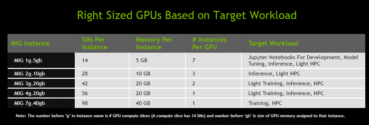
As a follow up to this work, we will study how to best use the A100 MIG computing resources by running the right type of workload on the right MIG instance sizes. See this table for an illustration of NVIDIA-recommended workload types for the different MIG sizes of the A100. We will use typical AI/ML workloads like inference, training, or Jupiter light training performed by data scientists during model development and other times to show how to avoid GPU underutilization by using smaller MIG instance sizes with minimal performance loss.
In addition, we will continue to keep track of the GPU Operator progress, paying particular attention to the auto-tuning/auto-slicing capabilities that are under discussion. These include how to find out which MIG instance size would be the best fit for running a given application and how to reconfigure the MIG-capable GPUs of the cluster to best serve the upcoming workload, given its MIG requirements. Stay tuned for the answer to these questions.